Welcome to Geography 104 In this section of our website, you will find helpful information and links related to the topics being discussed in class each week. The content of this section will be updated weekly.
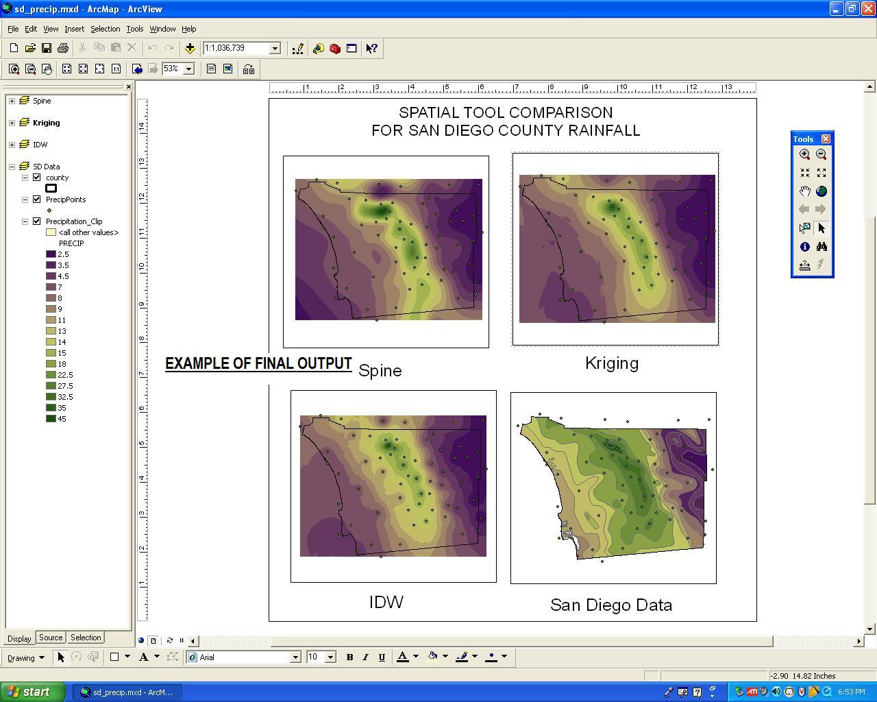
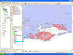
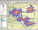
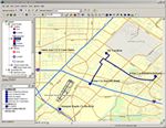
Although beginning students may not know much about GIS at the start of the semester, a successful student will be able to implement a GIS project from start to finish by the end of the semester. Here are a few examples of projects that students have created in this class in past semesters:
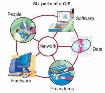
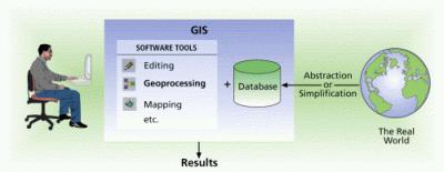
GIS DEFINITIONS GIS has been defined in several ways.....
1. " A powerful set of tools for storing and retrieving at will, transforming and displaying spatial data from the real world for a particular set of purposes." Peter Burrough
2. "Automated systems for the capture, storage, retrieval, analysis, and display of spatial data." Keith Clarke
3. "An information system that is designed to work with data referenced by spatial or geographic coordinates. In other words, a GIS is both a database system with specific capabilities for spatially-referenced data, as well as a set of operations for working with the data." Jack Estes
4. "A GIS is a special case of IS where the database consists of observations on spatially-distributed features, activities, or events which are definable in space as points, lines, and areas to retrieve data for ad hoc queries and analyses." Ken Duecker
From: Geographic Information Systems and Science, 2nd ed. Paul Longley, Michael Goodchild, David Maguire, and David Rhind
The Basics of GIS Kenneth E. Foote and Margaret Lynch, The Geographer's Craft Project, Department of Geography, The University of Colorado at Boulder
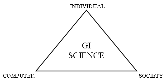
GEOGRAPHIC INFORMATION SCIENCE
The three elements of GI Science
Individual: Research dominated by cognitive science (the process of learning and knowing). Understanding spatial concepts, learning and reasoning about geographic data, and computer interaction.
Computer: Research about representation, adoption of new technologies, computation, and visualization.
Society: Research about issues of impacts and societal context.
GIS APPLICATIONS
Problem-solving applications
A. Objective or Goal Driven For example, problem-solving to maximize or minimize costs or distances
B. Tangible vs. Intangible For example, problem-solving that examines physical things that are directly measureable (tangible) like the quantity of water in a stream versus problem-solving that examines things that are not directly measurable such as assessing the quality of life or significance of environmental impacts (intangible).
C. Multiple Objectives For example, problem-solving that determines both the cost and the environmental impacts. This is often referred to as multi-criteria decision making.
GIS and related Geospatial Technologies are part of the High Growth Job Training Initiative "The High Growth Job Training Initiative is a strategic effort to prepare workers to take advantage of new and increasing job opportunities in high growth, high demand and economically vital sectors of the American economy. Fields like health care, information technology, and advanced manufacturing have jobs and solid career paths left untaken due to a lack of people qualified to fill them."
Note: If you are looking for the content that was previously in this section (from last week), it has been moved to the archived page. You can access the archive using the link in the column to the left titled, "Class Website Content".
Representing Geography
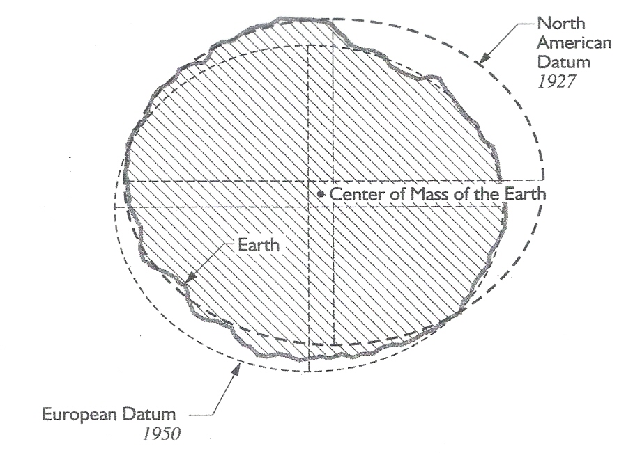
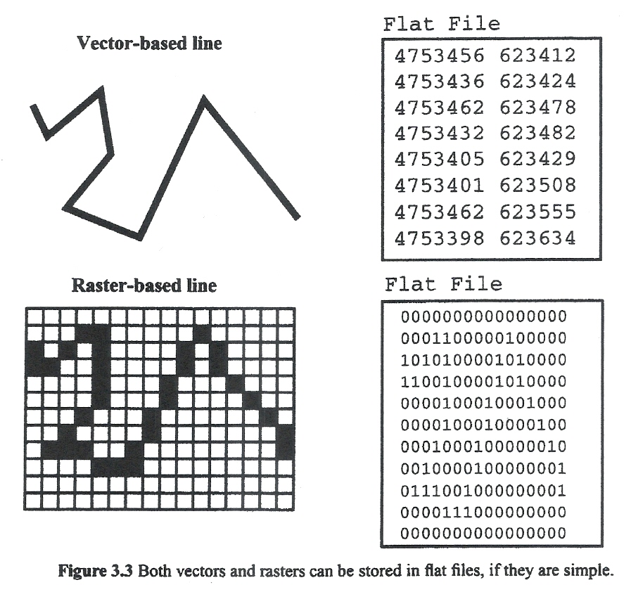
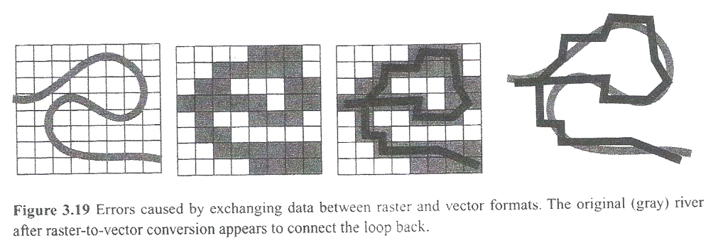
This week, we will take a look at how spatial information is transformed and represented. Topics of discussion will include datums, coordinate systems, and raster vs. vector data representation.
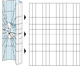
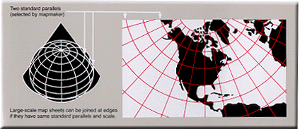
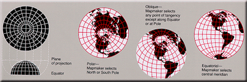
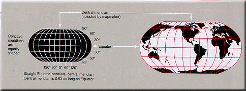
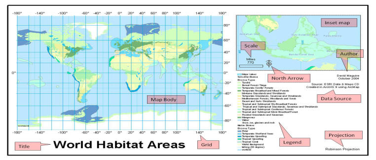
The Earth's image must be projected onto flat surfaces like computer screens and paper maps. These flat representations of the Earth are called “map projections.”
There are many types of map projections. No map projection is perfect. Any map projection will have some error in representing the Earth, but the inaccuracies can be reduced by choosing the appropriate map projections for specific needs.
Projecting reality from 3-dimensions to 2-dimensions.
The Magellan-Elcano Circumnavigation Route. Shown in the Raisz Armadillo Projection. Looks three-dimensional and equator is tilted upward.
The magellan-Elcano Circumnavigation Route. Shown in the Canters Minimum-Error Projection. Shape distortion is reduced.
The Voyager Flight. Shown in the Robinson Projection. The shapes of areas are well-preserved. Path is shown with minimal distortion
The Voyager Flight. Shown in the Oblique Lambert Azimuthal Equal-Area Projection. Emphasizes circular nature of flight. Flight path is not interrupted.
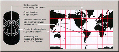
Sputnik I. Shown in the Miller Cylindrical Projection. Good for highlighting cyclical nature of orbiting path. But, increasingly distorts area poleward.
Sputnik I. Shown in the Snyder Cylindrical Satellite-Tracking Projection. Depicts satellite path as a set of straight lines. But, distorts area and shape poleward.
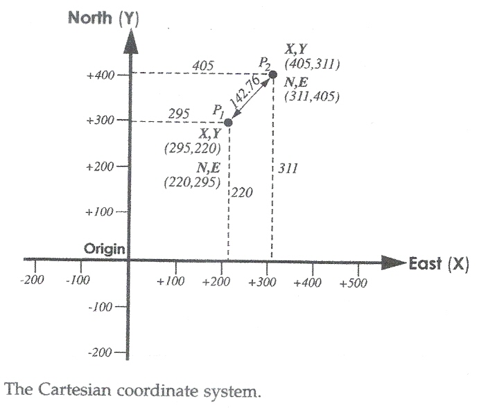
The essential problem of scale in a GIS is that all features are stored with precise coordinates (the computer stores numeric values), regardless of the precision of the original source data. Data which came from any mixture of scales can be displayed and analyzed in the same GIS project. The output of mixing data of differing scales can lead to erroneous or inaccurate conclusions.
Consider these two coordinates:
(125.875, 500.379) (126.000, 500.000)
Both coordinates are stored with the same precision (3 decimal places). If we ignore the 3 decimal places of precision, the 2 coordinates are identical, but if we use the full precision of the data, the coordinates are different. Depending on the scale at which you view these points, they will either look like a single point or they will look like 2 separate points. As you zoom in closer, the relative distance between the points will increase.
Using data from many different scales introduces these types of problems. The adage "A chain is only as strong as its weakest link" applies here; the accuracy and precision of measurements, maps, and models from a GIS are only as good as the least accurate and precise data source.
Geovisualization is the process of developing maps in GIS that are constructed and used as "windows into the database" to support queries, analysis, and editing of information.
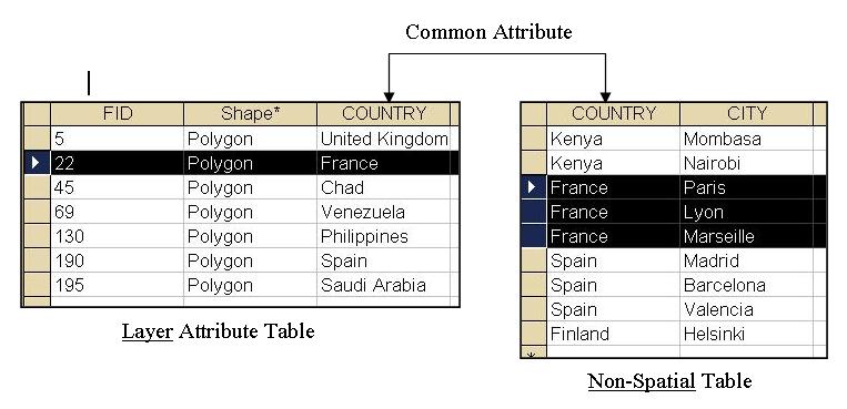
Tables and Attribute Data
Querying Data In Tables
Four Ways to get information about features:
Ø Identify Features: Click on a feature in the map with the Identify tool to display attribute information. [fastest way to get info about a single feature]
Ø Selecting Features Interactively: Click on features in the map to highlight them, then look at their records in the attribute table. [best for comparing several features]
Ø Selecting Features by Attributes: Write a Query [SQL] that automatically selects features that meet a certain criteria.
Ø Finding Features: Provide ArcMap with a piece of information (such as a name) to see which feature is belongs to.
Modifying Existing Tables
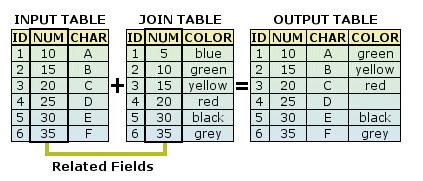
Joining, Relating, Linking, Hyperlinking Creating, and Importing Tables in GIS
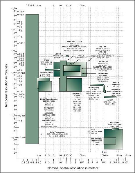
Spatial/Temporal Characteristics of Remote Sensing Systems
"Spatial and temporal characteristics of commonly used remote sensing systems and their sensors"From: Geographic Information Systems and Science, 2nd ed. Paul Longley, Michael Goodchild, David Maguire, and David Rhind. Originally From: Jenson, J.R. and Cowen, D.C. 1999 'Remote Sensing of urban/suburban infrastructure and socioeconomic attributes' PERS, 65, 611-622.
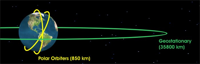
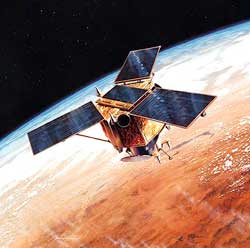
Polar Orbiting Satellites complete 14 orbits per day, thus covering the entire earth twice in a 24-hour period. They pick up the high-latitudes that are not covered by the Geostationary satellites. Their track runs nearly North to South passing close to both poles. They make back and forth swaths.
LANDSAT Bands 4-7 (.5-1.1ƛ) What spectral bands to I use for my study?
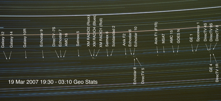
A time lapse of a small portion of the geostationary orbit taken from atop Kitt Peak in Arizona from 0230Z to 11Z on March 19, 2007. The lines represent star trails, while the bright dots mark the positions of geostationary satellites. Courtesy of Dave Dooling, National Solar Observatory. This image only accounts for 9% of all geostationary satellites orbiting Earth.
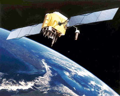
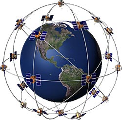
The space segment includes the satellites and the Delta rockets that launch the satellites from Cape Canaveral, in Florida. GPS satellites fly in circular orbits at an altitude of 10,900 nautical miles (20,200 km) and with a period of 12 hours. The orbits are tilted to the earth's equator by 55 degrees to ensure coverage of polar regions. Powered by solar cells, the satellites continuously orient themselves to point their solar panels toward the sun and their antenna toward the earth. Each of the 24 satellites, positioned in 6 orbital planes, circles the earth twice a day.
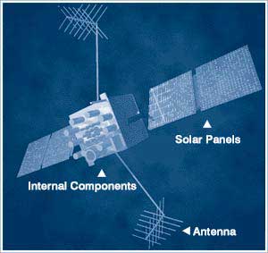
The satellites are composed of:
Solar Panels. Each satellite is equipped with solar array panels. These panels capture energy from the sun, which provides power for the satellite throughout its life.
External components such as antennas. The exterior of the GPS satellite has a variety of antennas. The signals generated by the radio transmitter are sent to GPS receivers via the L-band antennas. Another component is the radio transmitter, which generates the signal. Each of the 24 satellites transmits it's own unique code in the signal.
Internal components such as atomic clocks and radio transmitters. Each satellite contains four atomic clocks. These clocks are accurate to at least a billionth of a second or a nanosecond. An atomic clock inaccuracy of 1/100th of a second would translate into a measurement (or ranging) error of 1,860 miles to the GPS receiver.
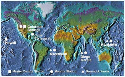
Master Control Station: The master control station, located at Falcon Air Force Base in Colorado Springs, Colorado, is responsible for overall management of the remote monitoring and transmission sites. GPS ephemeris being a tabulation of computed positions, velocities and derived right ascension and declination of GPS satellites at specific times, replace "position" with "ephemeris" because the Master Control Station computes not only position but also velocity, right ascension and declination parameters for eventual upload to GPS satellites.
Monitor Stations : Six monitor stations are located at Falcon Air Force Base in Colorado, Cape Canaveral, Florida, Hawaii, Ascension Island in the Atlantic Ocean, Diego Garcia Atoll in the Indian Ocean, and Kwajalein Island in the South Pacific Ocean. Each of the monitor stations checks the exact altitude, position, speed, and overall health of the orbiting satellites. The control segment uses measurements collected by the monitor stations to predict the behavior of each satellite's orbit and clock. The prediction data is up-linked, or transmitted, to the satellites for transmission back to the users. The control segment also ensures that the GPS satellite orbits and clocks remain within acceptable limits. A station can track up to 11 satellites at a time. This "check-up" is performed twice a day, by each station, as the satellites complete their journeys around the earth. Noted variations, such as those caused by the gravity of the moon, sun and the pressure of solar radiation, are passed along to the master control station.
Ground Antennas: Ground antennas monitor and track the satellites from horizon to horizon. They also transmit correction information to individual satellites.
The User Component
The user component consists of:
The user segment includes the equipment of the military personnel and civilians who receive GPS signals. Military GPS user equipment has been integrated into fighters, bombers, tankers, helicopters, ships, submarines, tanks, jeeps, and soldiers' equipment. In addition to basic navigation activities, military applications of GPS include target designation, close air support, "smart" weapons, and rendezvous.
With more than 500,000 GPS receivers, the civilian community has its own large and diverse user segment. Surveyors use GPS to save time over standard survey methods. GPS is used by aircraft and ships for enroute navigation and for airport or harbor approaches. GPS tracking systems are used to route and monitor delivery vans and emergency vehicles. In a method called precision farming, GPS is used to monitor and control the application of agricultural fertilizer and pesticides. GPS is available as an in-car navigation aid and is used by hikers and hunters. GPS is also used on the Space Shuttle. Because the GPS user does not need to communicate with the satellite, GPS can serve an unlimited number of users.
The aviation community is using GPS extensively. Aviation navigators, equipped with GPS receivers, use satellites as precise reference points to trilaterate the aircraft's position anywhere on or near the earth. GPS is already providing benefits to aviation users, but relative to its potential, these benefits are just the beginning. The foreseen contributions of GPS to aviation promise to be revolutionary. With air travel nearly doubled in the 21st Century, GPS can provide a cornerstone of the future air traffic management (ATM) system that will maintain high levels of safety, while reducing delays and increasing airway capacity. To promote this future ATM system, the FAA's objective is to establish and maintain a satellite-based navigation capability for all phases of flight.
The polynomial transformation uses a polynomial that is built upon control points and a least square fitting (LSF) algorithm. It is optimized for global accuracy but does not guarantee local accuracy. The polynomial transformation yields two formulas: one for computing the output x-coordinate for an input (x,y) location and one for computing the y-coordinate for an input (x,y) location. The goal of the least-square fit is to derive a general formula that can be applied to all points, usually at the expense of slight movement of the positions of the control points. The number of the non-correlated control points required for this method must be 3 for a first order, 6 for a second order, and 10 for a third order. The first-order polynomial transformation is commonly used to georeference an image.
Below is the equation to transform a raster dataset using the affine (1st order) polynomial transformation. You can see how six parameters define how a raster's rows and columns transform onto map coordinates.
Readings in Longley Text Chapter 12: Cartography and Map Production Chapter 13: Geovisualization
Work on Ch's 15 & 16 in Getting to Know ArcGIS Desktop
WEEK #8
GEOPROCESSING
Transformation Tools
Buffer and Intersect Operations
Pre-project Discussion
BUFFERING
Image By ESRI, INC.
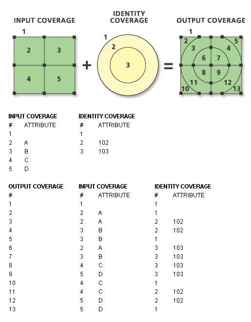
Identity Tool
Description: Computes the geometric intersection of two coverages. All features of the input coverage, as well as those features of the identity coverage that overlap the input coverage, are preserved in the output coverage.
Only those portions of identity coverage polygons that overlap the input coverage are saved in the output coverage. All input coverage polygons are saved in the output coverage. Input coverage arcs are split at their intersections with polygons of the identity coverage. The resulting arcs are used to build polygons using a process similar to Build with the POLY option.
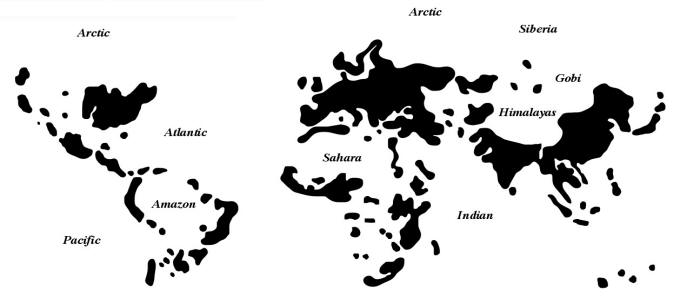
World Population Map (black indicates greater than 30 people per square mile)
Redrawn from William Bunge (The Continents and Islands of Mankind) Reproduced from "Making Maps"
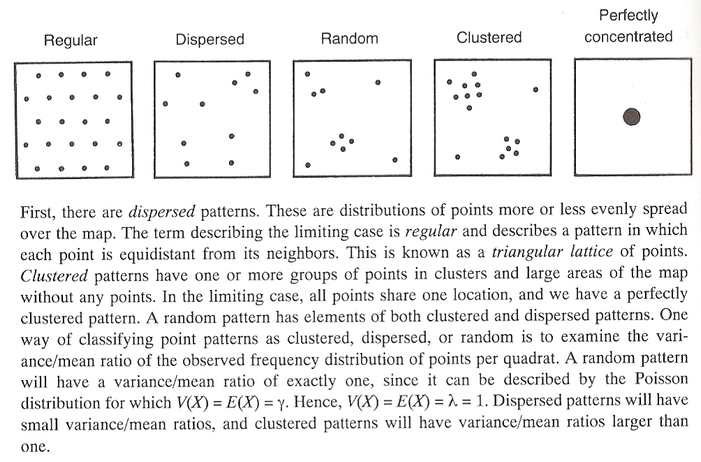
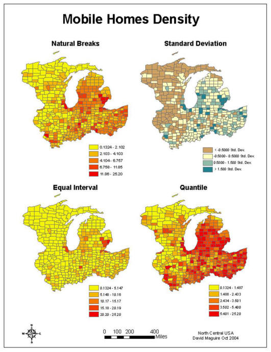
Data Classification
Natural Breaks (after George Jenks) Class breaks conform to gaps in data distribution. Minimizes variation within classes, and maximizes variation between classes.
Standard Deviation Class breaks based on a distance of standard deviation from the mean. Useful if data is distributed along a normal curve.
Equal Interval Equal distance between class breaks. The range of value that the class represents is the same for all classes.
Quantile Equal number of observations within each class. Class intervals can be significantly different in size with this classification.
Readings in Longley Text Chapter 16: Spatial Modeling with GIS
WEEK #11
Quiz #3 This Week
Project Proposal Due Next Week (April 17th)
Write in one page or less: 1. Topic 2. Research Question 3. Criteria 4. Data Availability 5. What new information will be produced? 6. Data Analysis (how will you generate new information to answer a question or address a problem).
3-D Analyst
WHY DISPLAY MY DATA IN 3D? Creating surfaces and 3D data can help you harness information from your GIS data that was not readily apparent in its 2D form.
ArcGIS 3-D Analyst provides the tools to work with surface data (real or hypothetical) to cartographically illustrate a 3rd dimension of the data (Z Value).
What is 3D Data?
3D data is data that has elevation or height information incorporated in its geometry. This information might be Z values of a feature class, cell values of a raster surface, or components of a TIN. In addition, there are ways to make 2D data render in 3D, for example, by using a surface as a source of base heights or using an attribute of a feature that contains elevation information. (ESRI, Inc.)
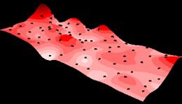
Surface Model of Chemical Concentrations Across an Area. Image From ESRI, Inc.
Two types of data surface models can be used:
1. Raster Data Raster format is used to store image data, thematic data, and surface data. Raster surfaces are stored in a GRID format. A grid format consists of a rectangular array of uniformly-spaced cells that have z-values. The image below illustrates a higher precision grid on the left and a lower precision grid on the right.
Grid with fine resolution on the left and coarse resolution on the right. Image from ESRI, Inc.
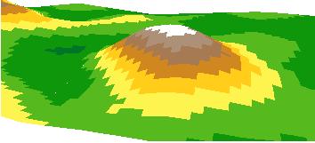
Grid in Perspective View. Image from ESRI, Inc.
The "Z" value field consists of an additional attribute that is stored in each cell and provides information for the 3rd dimension.
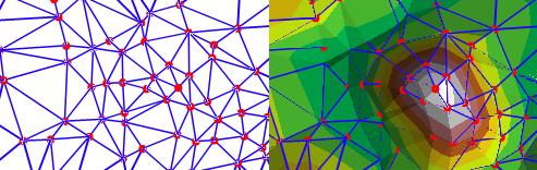
2. TIN Data
A TIN (Triangulated Irregular Network) consists of vertices that are triangulated and connected with a series of edges to form a network of triangles.
An example of a Triangulated Irregular Network. Image From ESRI, Inc.
Nodes can be placed irregularly across these surfaces that will create irregular sized and shaped triangles. Consequently, a TIN can have higher resolution in areas where more detail is needed. (ie: The resolution is variable across the surface) TIN's are typically used for high-precision modeling and often require more intensive computer hardware processing.
Many surface models are available in the data world for use. OR You can create your own using Interpolation and Triangulation Methods.
3D-Modelling can be performed using tools within the ArcGIS 3D Analyst.
3D ANALYST LETS YOU:
Convert TIN's to features and rasters
Create 3D features from functional surfaces by extracting height information
Interpolate information from rasters
Mathematically manipulate rasters
Reclassify rasters
Derive height, slope, aspect, and volumetric information from TIN's and rasters
"Geocoding is the process of assigning a location, usually in the form of coordinate values (points), to an address by comparing the descriptive location elements in the address to those present in the reference material." ESRI, Inc.
"ArcGIS Network Analyst is a powerful extension that provides network-based spatial analysis including routing, travel directions, closest facility, and service area analysis. ArcGIS Network Analyst enables users to dynamically model realistic network conditions, including turn restrictions, speed limits, height restrictions, and traffic conditions, at different times of the day." ESRI, Inc.
If you have not already submitted your proposal, do so immediately!
Proposal Guidelines Write in one page or less: 1. Topic 2. Research Question 3. Criteria 4. Data Availability 5. What new information will be produced? 6. Data Analysis (how will you generate new information to answer a question or address a problem).
WEEK# 13
GPS TO GIS EXERCISE THIS WEEK
Bring notes and handouts to class. You will use a GPS device to collect data in the field. Then, that data will be imported into GIS and manipulated to generate new information to answer a question. Some of the tasks required of you will include:
1. Data Collection (including metadata) with GPS 2. Download data into computer 3. Manage table of data and data formats 4. Prepare data for input to ArcGIS 5. Add metadata as attributes into a table 6. Creation of a new shapefile in ArcCatalog
7. Utilization of ArcEditor to add features to the new shapefile 8. Use Spatial Analyst tools to extract new information from newly created features 9. Cartographically represent data in a meaningful and appropriate way 10. Design a presentation layout, complete with data frames, legend, title, summary, etc.
Write in one page or less: 1. Topic 2. Research Question 3. Criteria 4. Data Availability 5. What new information will be produced? 6. Data Analysis (how will you generate new information to answer a question or address a problem).
WEEK# 14
Project Work This Week
SAVE YOUR WORK OFTEN!
Be prepared to work on your project during each of the remaining class meetings. Take advantage of lab time and maximize your productivity. Finalize your project and print on May 21st.
Note: It is required that you save a copy of your final poster in PDF format and email the PDF to your instructor.
To organize the steps you initiate to complete your project, you may want to create a flow chart. See below for a few examples.
Timeline This Week: Project Work (finalize data collection, initiate data analysis) Next Week (5/14): Project Work (complete data analysis, initiate poster layout) In 2 Weeks (5/21): Finish poster layout, symbology, and cartography. Print poster.
FOR THE FINAL CLASS MEETING PRIOR TO PRESENTATIONS
1. If not already completed, finish processing by 8:00pm. If you are not done with the processing by 8:00pm, then begin designing the layout of your poster with the data and steps that you did accomplish up to 8:00pm. 2. Complete layout of poster. 3. Have someone proof-read your poster for errors, suggestions, etc. (required) 4. Create a PDF version of your poster and email to your instructor. 5. Print your poster with the assistance of your instructor or the acting T.A.
Project Tutorial Examples A method you can use to create a history of the procedures you implement to address your criteria and generate results. An outline (tutorial) documenting the various steps you take can be useful later when you have to explain your project from start to finish on your final poster. You won't turn in this outline. It's just to be used as a way to document your procedures in order from start to finish so that you can keep track of what you are doing and refer back to it later.
Timeline This Week: Project Work (complete data analysis, initiate poster layout) Next Week: (5/21): Finish poster layout, symbology, and cartography. Print poster.
PROJECT PRESENTATIONS MAY 28th at 7PM
SAVE YOUR WORK OFTEN!
Be prepared to work on your project during each of the remaining class meetings. Take advantage of lab time and maximize your productivity. Finalize your project and print on May 21st.
Note: It is required that you save a copy of your final poster in PDF format and email the PDF to your instructor.
To organize the steps you initiate to complete your project, you may want to create a flow chart. See below for a few examples.
FOR THE FINAL CLASS MEETING PRIOR TO PRESENTATIONS
1. If not already completed, finish processing by 8:00pm. If you are not done with the processing by 8:00pm, then begin designing the layout of your poster with the data and steps that you did accomplish up to 8:00pm. 2. Complete layout of poster. 3. Have someone proof-read your poster for errors, suggestions, etc. (required) 4. Create a PDF version of your poster and email to your instructor. 5. Print your poster with the assistance of your instructor or the acting T.A.
Project Tutorial Examples A method you can use to create a history of the procedures you implement to address your criteria and generate results. An outline (tutorial) documenting the various steps you take can be useful later when you have to explain your project from start to finish on your final poster. You won't turn in this outline. It's just to be used as a way to document your procedures in order from start to finish so that you can keep track of what you are doing and refer back to it later.